Ashley Hendrickson
- Software Engineer
Linear Regression.
Linear regression is a statistical approach to modeling the relationship between a scalar response and one or more explanatory variables. (It’s basically a line of best fit). This is the first basic concept in data science.
With a single input, we can model our data using

With multiple inputs, we will use the following equation to measure the dot product:

We can use Linear Regression to make a prediction when we have data that is linear.
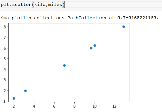
For example – say you want to convert kilometers to miles. If you plot this – you would see a direct linear correlation between kilometers and miles.

First, let’s import our libraries we will be using tensorflow for our model. We will use numpy to properly format our data and matplotlib.pylot to print a graph

We will use the following data for this example. Each point describes the distance in respect to the other point. For example, 10 kilometers is equivalent to 6.21371 miles.
To confirm the data is linear we can plot:

The data happens to be perfectly linear, but it doesn’t have to be. We just need to be able to properly describe our data with a line of best fit.
First we will instantiate our model:
Since our function has a one -to- one correlation-meaning for every x there is a –y- we can use a sequential model to map our data. Sequential models are only appropriate when our model has one input, is liner, and doesn’t require layer sharing.
Dense is the regular deeply-connected neural network layer. It is the most commonly used layer. It creates a matrix with biases created out of layers if the input to layer is greater than two. It then computes the dot product between the input and the kernel.
The unit is a positive Integer, representing the dimensionality of the output.
The model needs to know what input shape it should expect for a sequential model. The input shape returns as an integer shape, tuple, or list of shape tuples, one tuple per input tensor.
Next we will compile the model:
The purpose of the loss function is to compute the quantity that our model should seek to minimize during training. The mean squared error just computes the mean squared error.
Adam is just an optimizer that implements the Adam algorithm which is a stochastic gradient descent method that is based on adaptive estimation of first-order and second-order moments. The current value it holds is our learn rate: if we don’t provide it with a value it will default to 0.001
Now we will train our model:
Every time our network passes a batch through the network, it generates a prediction result which then weighs them against biases.
Epochs refers to one cycle through the full training dataset. If we lower the epochs, our accuracy and precision decline but the model will train faster, the opposite is true for the inverse.
Verbose isn’t important- it just prints the time it took to run each epoch.
Finally, we will try to make a prediction with our model:
Let’s see what our predication is for 20 kilometers converted to miles:

The correct answer approximately 12.427423845
This is 99.99978% correct. Note that this is only because our data is perfectly linear. If our data wasn’t perfectly linear and more messy we would get a prediction that would be less accurate. If you’re wondering why our data isn’t 100% correct, we rounded our initial values in both arrays to the 4th decimal place. We could have achieved more accuracy if we gave more exact values. Notice we never gave our model any indication of what our formula might be. Instead our model was able to learn and build its own formula. This might not be too impressive but it’s a basic fundamental that will be important to understand when building upon in order to make more complex concepts.

